
Unlock the power of Transformer Networks and learn how to build your own GPT-like model from scratch. In this in-depth guide, we will delve into the theory and provide a step-by-step code implementation to help you create your own miniGPT model. The final code is only 400 lines and works on both CPUs as well as on the GPUs. If you want to jump to the implementation here is the GitHub repo.
The era of Transformers
Transformers are revolutionizing the world of artificial intelligence. This powerful neural network architecture, introduced in 2017, has quickly become the go-to choice for natural language processing, generative AI, and more. With the help of transformers, we've seen the creation of cutting-edge AI products like BERT, GPT-x, DALL-E, and AlphaFold, which are changing the way we interact with language and solve complex problems like protein folding. And the exciting possibilities don't stop there - transformers are also making waves in the field of computer vision with the advent of Vision Transformers.
Transformers are even considered as a future single neural network architecture for multimodal inputs (text, image, video, audio), and thus converging all the other architectures into one: Gato, a multi-modal, multi-task, multi-embodiment generalist agent developed by DeepMind in 2022.
Before Transformers, the world of AI was dominated by convolutional neural networks for computer vision (VGGNet, AlexNet), recurrent neural networks for natural language processing and sequencing problems (LSTMs, GRUs) and Generative Adversarial Networks (GANs) for generative AI. As of 2017, CNNs and RNNs accounted for 10.2% and 29.4% respectively of papers published on pattern recognition. But already in 2021 Stanford researchers called transformers “foundation models” because they see them driving a paradigm shift in AI.
Transformers combine some of the benefits traditionally seen with convolutional neural networks (CNNs) and recurrent neural networks (RNNs).
One benefit that transformers share with CNNs is the ability to process input in a hierarchical manner, with each layer of the model learning increasingly complex features. This allows transformers to learn highly structured representations of the input data, similar to how CNNs learn structured representations of images.
Another benefit that transformers share with RNNs is the ability to capture dependencies between elements in a sequence. Unlike CNNs, which process input in a fixed-length window, transformers use self-attention mechanisms that allow the model to directly relate different input elements to each other, regardless of their distance in the sequence. This allows transformers to capture long-range dependencies between input elements, which is particularly important for tasks like natural language processing where it is necessary to consider the context of a word in order to accurately understand it.
Andrej Karpathy has summarised the power of Transformers as a general-purpose differentiable computer. It's very powerful in a forward pass, because it can express very general computation. The nodes store vectors and these nodes look at each other and they can see what's important for their computation in the other nodes. On the backward pass it is optimisable with the residual connections, layer normalisation and softmax attention. So you can optimise it using the first-order methods like gradient descent. And lastly you can run it efficiently on modern hardware (GPUs), which prefers lots of parallelism.
Remarkably, the Transformer architecture is very resilient over time. The Transformer that came out in 2017 is basically the same as today except that you reshuffle some of the layer normalisations. Researchers are making training datasets much larger, evaluation much larger, but they are keeping the architecture untouched, which is remarkable.
Attention is all you need

The new architecture was proposed in the article Attention Is All You Need, published in 2017. The article described a new type of neural network architecture called the Transformer, which is based on a self-attention mechanisms unlike traditional convolutional or recurrent neural networks.
The original paper describes an encoder-decoder architecture for Transformer to solve the translation problem.
In this article, however we will focus on the decoder-only architecture as we will be building a GPT like model, i.e. we are solving a sentence completion task rather than a translation task described in the paper.
For the translation task you need to encode the input text first and have a cross-attention layer with the translated text. In the sentence completion only the decoder part is necessary, so let's focus on it.
Encoder-decorder stack
To begin with, let's recall the encoder-decoder architecture. The language models could be roughly categorised into Encoders only (BERT) - they have only the encoder blocks, Decoders only (GPT-x, PaLM, OPT) - only the decoder blocks and Encoder-Decoder (BART, T0/T5). Essentially, the difference boils down to the task that you are trying to solve:
Encoder only architectures (like BERT) solve the task of predicting the masked word in a sentence. So the attention can see all the words before and after this masked word. This has a term "masked language modelling". The encoder architecture is typically used for language modeling tasks that involve encoding a sequence of input tokens and producing a fixed-length representation, also known as a context vector or embedding, which summarizes the input. This context vector can then be used by a downstream task, such as machine translation or text summarization. BERT model is an good example.
For decoder and encoder-decoder architectures the task is to predict the next token or set of tokens, i.e. given tokens [0, ..., n-1] predict n. These architectures are used for language modelling tasks that involve generating a sequence of output tokens based on an input context vector.
In the article Attention Is All You Need, the encoder and decoder are represented by six layers (the number can be any, for example, in BERT there are 24 encoder blocks).

Each encoder consists of two layers: Self-Attention and Feed Forward Neural Network. The input data of the encoder first passes through the Self-Attention layer. This layer helps the encoder look at other words in the input sentence when it encodes a particular word. The results of this layer are fed to the fully connected layer (Feed Forward Neural Network).
As the model processes each token (each word in the input sequence), the Self-Attention layer allows it to search for hints in the other tokens in the input sequence that may help improve the encoding of that word. In the fully connected layer, the Feed Forward Neural Network has no interaction with other words, and therefore various chains can be executed in parallel as they pass through this layer. This is one of the main characteristics of Transformers, which allows them to process all words in the input text in parallel.
A few more words about Attention
We actually calculate “attentions” unconsciously as we speak. You constantly care about what “she”, “it” , “the”, or “that” refers to. Imagine a sentence "I've never been to Antarctica, but it is on my wish list". We know that "it" refers to "Antarctica".
The authors of the article Attention Is All You Need introduce a concept of Query/Key/Value vectors. A good analogy is a retrieval system. For example, when you search for videos on Youtube, the search engine will map your Query (text in the search bar) against a set of Keys (video title, description, etc.) associated with the videos in their database, and give you a result with the best matched videos (Values).
In our example, let's say we want to compute the self-attention for the word "it" in the sentence "I've never been to Antarctica, but it is on my wish list". The process would involve creating matrices Q, K, and V for the input sentence, where q (row in matrix Q) represents the query vector for the word "it", K represents the key matrix for all the words in the sentence, and V represents the value matrix for all the words in the sentence.
The self-attention for "it" would then be computed as the dot product of Q and K, divided by the square root of the length of K, followed by a dot product with V. This would result in a weighted sum of the values in V, with the weights determined by the relevance of each word in the sentence to the query "it". In this case, the self-attention for "it" would likely be higher for the word "Antarctica", since they are related.
How are these Query (Q), Key (K) and Value (V) vectors generated?

A simple answer is by vector-to-matrix multiplication with three different matrices (WQ, WK, WV). The vector (xn) in this case would be a word embedding of the input token (or output of the previous attention layer). The matrices WQ, WK, WV are initially randomly initialized weight matrices. Their task is to reshape the input vector into a smaller shape representing Query, Key and Value vectors (q, k, v).

Let's come back to a shorter prompt "Hello world" and see how it will be process by the Transformer architecture. We have two embedded input words: x0 as an embedding for "Hello" and x1 as an embedding for "world".
And we have vectors q, k and v for each of these two words. These vectors are generated by multiplying embedding vector of the word and the weight matrix W:
Same logic but in a matrix form
We can present the same Query, Key and Value vectors (q, k, v) in a matrix form for all the input tokens (words) at once. And that's the power of Transformer architecture - we can process all input words at once.

X [N × dmodel] - is embeddings matrix for the input words (in our case - embeddings of the two words "Hello" and "world").
W [dmodel × dk] - randomly initialized weight matrices.
Q [N × dq] - the matrix of query vectors.
K [N × dk] - the matrix of key vectors.
V [N × dv] - the matrix of value vectors.
N - number of tokens in an input sequence;
dv - dimension of values vectors;
dk = dq - dimension of keys and queries vectors;
dmodel - dimension of the hidden layers or the dimension of the token embeddings;
h = number of heads of multi-head attention (discussed later);
In the paper the dmodel = 512 (in our illustration - 5 squares), dk = dq = dv = dmodel/h = 64 (3 squares)
Now let's compute the Attention matrix
Once we get our matrices Q, K and V, we can now compute the matrix for attention scores. The score determines how much focus we apply on other parts of the input sentence as we encode a word at a certain position.

Step by step:
First step - multiplying Q and transposed Key matrix. Each query vector ("Hello" and "world") is DotProduct-ed with the word vectors of each of the keys. This is similar to the retrieval process, when you find the best matching YouTube video based on the query and the keys like video title, description. The result would be a matrix N*N where the N is the size of the input sentence (number of tokens). In our case it's 2*2.

m0 - weights to compute attention for the first word m1 - similar for the second word
Here m0 = (q0*k0, q0*k1) represents the attention score vector of word "Hello". In essence it says relevance of the first word in the sentence ("Hello") to the query "Hello" is q0*k0 and the relevance of the second word in the sentence ("world") to the query "Hello" is q0*k1. Similarly m1 = (q1*k0, q1*k1) represents the attention score vector of word "world". We also scale the resulting matrix values by square root of the size of K in order to have more stable gradients.Second step - take a softmax in each row of the resulting matrix (in our case of vectors m0 and m1). Softmax normalizes the scores so they’re all positive and add up to 1 in a row.
Third step - is to sum up the weighted value vectors. This produces the output of the self-attention layer at this position.
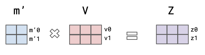
So we have our normalised matrix of weights m' from the Step 2. We then get the self-attention as the weighted sum of the Values vectors. This final step results in a single output word vector representation of each input word.


Now we can repeat this logic by adding a new attention block to the encoder. We can take the resulting matrix Z (a.k.a “hidden vectors”), and considering it as inputs to the new attention layer, which will output Z1 with the new word vectors of its own. In the original paper the encoder is represented by six such blocks, but it could be any number (for example, in BERT there are 24 encoder blocks).
Summarising it by pointing out that each token (query) is free to take as much information using the dot-product mechanism from the other words (values), and it can pay as much or as little attention to the other words as it likes by weighting the other words with Keys.
Self-attention implementation
class AttentionHead(nn.Module):
    """
    One head of the self-attention layer
    """

    def __init__(self, head_size, num_embed, block_size):
        super().__init__()
        self.key = nn.Linear(num_embed, head_size, bias=False)
        self.query = nn.Linear(num_embed, head_size, bias=False)
        self.value = nn.Linear(num_embed, head_size, bias=False)
        # tril is a lower triangular matrix. it is not a parameter
        # of the model, so we assign it to the module using register_buffer
        self.register_buffer("tril", torch.tril(torch.ones(block_size, block_size)))

    def forward(self, x):
        B, T, C = x.shape
        k = self.key(x)
        q = self.query(x)
        # compute attention scores
        # (B, T, C) @ (B, C, T) -> (B, T, T)
        # we need to transpose k to match q
        wei = q @ k.transpose(-2, -1) * C**-0.5
        # Tril matrix (lower triagular matrix) is used to mask
        # future positions (setting them to -inf) so that the
        # decoder "learns" to predict next words
        wei = wei.masked_fill(self.tril[:T, :T] == 0, float("-inf"))  # (B,T,T)
        wei = F.softmax(wei, dim=-1)  # (B,T,T)
        # weighted aggregation of the values
        v = self.value(x)
        out = wei @ v  # (B,T,T) @ (B,T,C) ---> (B,T,C)
        return out
Multi-head Attention
The attention mechanism is further improved by averaging several attentions together. This operation is similar in some way to using different filters in the CNN. Multi-head attention allows the model to jointly attend to information from different representation subspaces at different positions.

Note: the dimension of WO is h*dv × dmodel , so that dimensions of the resulting matrix Z is N × dmodel.
Multihead Attention implementation
class MultiHeadAttention(nn.Module):
    """
    Multiple Heads of self-attention in parallel
    """

    def __init__(self, num_heads, head_size, num_embed, block_size):
        super().__init__()
        self.heads = nn.ModuleList(
            [
                AttentionHead(
                    head_size=head_size,
                    num_embed=num_embed,
                    block_size=block_size,
                )
                for _ in range(num_heads)
            ]
        )
        self.proj = nn.Linear(num_embed, num_embed)

    def forward(self, x):
        # output of the self-attention
        out = torch.cat([h(x) for h in self.heads], dim=-1)
        # apply the linear projection layer
        out = self.proj(out)
        return out
Residuals & Layer normalisation
In the transformer architecture, the residual connections are a type of shortcut connection that allows the information to bypass one or more layers of the network. Residual connections (-->) are employed around each of the two sub-layers, followed by layer normalization.

Residual connections are used to help address the problem of vanishing gradients, which can occur when the gradients of the network become very small and it becomes difficult for the network to learn effectively. By allowing the information to bypass some of the layers, the residual connections can help to maintain the magnitude of the gradients as the information flows through the network, making it easier for the network to train.
Residual connection implementation and Feed forward
class FeedForward(nn.Module):
    """
    A simple linear layer followed by ReLu
    """

    def __init__(self, num_embed):
        super().__init__()
        self.net = nn.Sequential(
            # in the Attention is All You Need paper
            # authors are using the size of the ffwd layer 2048
            # and the output of the model is 512
            # so we apply the same factor of 4
            nn.Linear(num_embed, 4 * num_embed),
            nn.ReLU(),
            # apply the linear projection layer
            nn.Linear(4 * num_embed, num_embed),
        )

    def forward(self, x):
        return self.net(x)

class TransformerBlock(nn.Module):
    """
    This calss will group together MultiHead Attention and
    FeedForward NN, so that we can copy it in Transformer
    """

    def __init__(self, num_heads, block_size, num_embed):
        super().__init__()
        head_size = num_embed // num_heads
        self.sa = MultiHeadAttention(
            num_heads=num_heads,
            head_size=head_size,
            num_embed=num_embed,
            block_size=block_size,
        )
        self.ffwd = FeedForward(num_embed=num_embed)
        # add the layer normalization
        self.ln1 = nn.LayerNorm(num_embed)
        self.ln2 = nn.LayerNorm(num_embed)

    def forward(self, x):
        # "x +" is the skip (or residual) connection
        # it helps with optimization
        # also we apply layer normalization before self-attention
        # and feed-forward (a reshufle from original paper)
        x = x + self.sa(self.ln1(x))
        x = x + self.ffwd(self.ln2(x))
        return x
Generation
The transformer predicts the next word having the context of all the previous words. This is done by a Linear and a Normalisation layers.
The Linear layer projects the output of the stack of decoders into a much larger vector called the logits vector. If the model has learnt a dictionary of 100,000 words (like GPT-3) from its training dataset, the logits vector will have 100,000 scores for each word.
The Softmax then turns those scores into probabilities (all positive and add up to 1). The cell with the highest probability is chosen, and the word associated with it is produced as the output for this iteration.
Implementation of the Transformer with generate method to predict next words
class Transformer(nn.Module):
    def __init__(self, **kwargs):
        super().__init__()
        # a simple lookup table that stores embeddings of a fixed dictionary and size
        # each token directly reads off the logits for the next token from a lookup table
        # see more: https://pytorch.org/docs/stable/generated/torch.nn.Embedding.html
        self.vocab_size = kwargs.get("vocab_size", 100)
        self.num_embed = kwargs.get("num_embed", 32)
        self.block_size = kwargs.get("block_size", 8)
        self.num_heads = kwargs.get("num_heads", 4)
        self.num_layers = kwargs.get("num_layers", 4)
        # each token reads the logits for the next token from a lookup table
        self.token_embedding_table = nn.Embedding(self.vocab_size, self.num_embed)
        # each position from 0 to block_size-1 will get its embedding
        self.position_embedding_table = nn.Embedding(self.block_size, self.num_embed)
        self.blocks = nn.Sequential(
            *[
                TransformerBlock(
                    num_heads=self.num_heads,
                    block_size=self.block_size,
                    num_embed=self.num_embed,
                )
                for _ in range(self.num_layers)
            ]
        )
        # we add the layer norm before the Linear layer
        self.ln_f = nn.LayerNorm(self.num_embed)
        self.lm_head = nn.Linear(self.num_embed, self.vocab_size)

    def forward(self, idx, targets=None):
        B, T = idx.shape
        # idx and targets are (B,T) tensor of integers
        # the token_emb is (B, T, C), C = NUM_EMBED
        token_emb = self.token_embedding_table(idx)
        # (T, C)
        posit_emb = self.position_embedding_table(torch.arange(T, device=DEVICE))

        x = token_emb + posit_emb
        # apply one head of self-attention
        x = self.blocks(x)
        # (B, T, vocab_size)
        logits = self.lm_head(x)
        # compute the loss
        if targets != None:
            # cross_entropy accepts inputs in a (batch_size, num_classes)
            # so we need to reformat our logits dimensions to
            # (batch_size * time, dim_vocabulary), time = block_size
            B, T, C = logits.shape
            logits = torch.reshape(logits, (B * T, C))
            targets = torch.reshape(targets, (B * T,))
            loss = F.cross_entropy(logits, targets)
        else:
            loss = None
        return logits, loss

    def generate(self, idx: torch.Tensor, max_new_tokens: int, block_size: int):
        # idx is (B, T) array of indices in the current context
        for _ in range(max_new_tokens):
            # crop the context too the  last block_size tokens
            # because tokens don't communicate between blocks
            idx_crop = idx[:, -block_size:]
            # get the predictions
            logits, loss = self.forward(idx_crop)
            # focus only on the last time step
            logits = logits[:, -1, :]  # becomes (B, C)
            # apply softmax to get probabilities
            probs = F.softmax(logits, dim=-1)  # (B, C)
            # sample from the distribution with probabilities probs
            idx_next = torch.multinomial(probs, num_samples=1)  # (B, 1)
            # append sampled index to the running sequence
            idx = torch.cat((idx, idx_next), dim=1)  # (B, T+1)
        return idx
Training process
As discussed before, with a GPT-like model we are trying to predict the next word having the context. In practice it looks the following way:
We define
xas a chunk of text starting from a random index and the chunk is the size block_size.We define
ythe same way, but this time this chunk of words is shifted one word to the right ofx.This way for each position in
xwe have a prediction of the next word in the same position ofy. This is our target.Finally, we actually take a batch of these random chunks of data and we stack them together (torch.stack) to process in parallel.
def get_batch(data: list[str], block_size: int, batch_size: int):
    ix = torch.randint(len(data) - block_size, (batch_size,))
    x = torch.stack([data[i : i + block_size] for i in ix])
    # y is x shifted one position right - because we predict
    # word in y having all the previous words as context
    y = torch.stack([data[i + 1 : i + block_size + 1] for i in ix])
    return x, y
The rest works similar to any other neural network:
Forward pass: we initialise randomly all the matrices, attention layers and weights of the fully-connected layers. After the first forward pass we get a vector in the last Softmax layer: [0.2, 0.2, 0.36, 0.03, 0.01, ....]. So we can predict the first word - the word with id=2 (0.36).
logits, loss = model.forward(xb, yb)Loss calculation: now we can compute the cross-entropy loss between the predictions and the target. Suppose the actual next word was on the position id=3 (we predicted id=2), then the loss would be:


Backward pass (a.k.a the back-propagation phase): The gradients of the loss with respect to the model parameters are calculated using backpropagation. We won't describe it here as the logic is similar to any other neural network.
optimizer.zero_grad(set_to_none=True) loss.backward()Optimization: The model parameters are updated in the direction that minimizes the loss, using an optimization algorithm such as stochastic gradient descent (SGD) or Adam.
optimizer.step()Repeat: The process of making forward and backward passes and optimizing the model parameters is repeated for multiple epochs until the model reaches satisfactory performance on the training data.
Evaluation: The model is evaluated on a separate validation set to assess its generalization performance and identify any overfitting. The model may be further fine-tuned based on the validation performance.
Note: please, checkout the GitHub repo for the full code with helper functions in utils.py.
for step in range(MAX_ITER):
    loss = estimate_loss(data=train_data, model=model)
    print(f"step {step:10} | train loss {loss_train:6.4f}")
    # sample a batch of data
    xb, yb = get_batch(data=train_data, block_size=BLOCK_SIZE, batch_size=BATCH_SIZE)
    logits, loss = model.forward(xb, yb)
    # zero_grad() method sets the gradients
    # of all parameters in the optimizer to zero
    optimizer.zero_grad(set_to_none=True)
    # backward() method on the loss variable calculates the gradients
    # of the loss with respect to the model's parameters.
    loss.backward()
    # step() method on the optimizer updates the model's parameters
    # using the calculated gradients, in order to minimize the loss.
    optimizer.step()
You can validate your model with a simple script to generate a random sequence of words starting from any random prompt:
# generate some output based on the context
context = torch.zeros((1, 1), dtype=torch.long, device=DEVICE)
print(
    decode(
        enc_sec=m.generate(idx=context, max_new_tokens=100, block_size=BLOCK_SIZE)[0],
        tokenizer=tokenizer,
    )
)