There’s a lot of talk about machine learning nowadays. A big topic – but, for a lot of people, covered by this terrible layer of mystery. Like black magic – the chosen ones’ art, above the mere mortal for sure. One keeps hearing the words “numpy”, “pandas”, “scikit-learn” - and looking each up produces an equivalent of a three-tome work in documentation.

I’d like to shatter some of this mystery today. Let’s do some machine learning, find some patterns in our data – perhaps even make some predictions. With good old Python only – no 2-gigabyte library, and no arcane knowledge needed beforehand.
Interested? Come join us.
1. Introduction

So, there is a game. A rather popular game - The Binding of Isaac, they call it. It’s a simple concept – you wander the basement and collect things. Depending on the nature of the things you collect, the game may become easier or harder. There is some strategy involved.

There is also a man. An avid player of the game – over a thousand sessions, each spanning half an hour (or even more!). A veteran of both The Binding of Isaac, and of light-hearted commentary about his personal life. If that is your sort of thing, I heavily recommend his older videos. Here is a link.
There is also a convenient surprise.
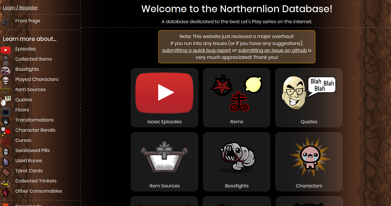
Devoted fans of our internet personality have erected a comprehensive database in his glory. Each episode (and is there a lot of them) is meticulously charted in a SQL table, and a couple of simple queries give us information on just about anything this man may have encountered during his playthrough. Here is a link, if this interests you. Now let us use this coincidence to our advantage.
A man runs through a computer-generated basement every day, collecting junk on his way. Every day, the recording is uploaded onto YouTube for people to enjoy. A thumb pointed up, or a thumb pointed down – the crowd judges the basement runner. Was it an interesting watch? That usually depends on the personal charm and charismatic dialogue of Mr. Northernlion himself... but charisma, the database does not store as a value. It does, however, store the items he picked up.
The question arises naturally – what items make a video interesting?
We can find out.
2. Preparing for the task
Before diving into theory, let’s talk a little bit about how to import the Northernlion devotees’ database into our favourite programming language.

If your favourite programming language is not Python, it should at least be C++. They are both very beautiful languages.
What do we want?
We want a simple, comprehensive translation of the things we see in the SQL dump we have downloaded into a big pile of examples. An example is a pair of all the items that we have gotten in a video, and the rating of that video on YouTube. We’ll talk more about this in the next chapter, once we start talking about machine learning concepts.
Here’s an example (warning, complicated data structure ahead):

That was a joke. The structure is not complicated at all.
We have a tuple. In it, the video ID (decorative), a counter (dictionary – item vs how much of it have we picked up), and the amount of likes the video has.
And also, we have a file 21.5 megabytes in size.
How do we make the second into the first?
Plan A: SQLite 3
Python is a great language. One of the things that makes it so is the extensive standard library. The unittest module, for one – a thing to write odes to. But that’s not our goal today. Let us talk about the module known as sqlite3.
The general idea of a SQL database is a specially designated server, a server that lives and breathes to fulfil all the requests for data that are sent to it from our side. It’s not the best paradigm, if you do not want to host a server.
In case you don’t (a common case), people like you are saved by something called SQLite 3 – not only an alternative paradigm, but also a trusted friend. Instead of a special server, SQLite operates on a simple file that contains the essence of our base. And that file can be operated using Python’s standard library, too! It is a very pleasant experience, if you do not want to host a server.
But, alas, our file is not a SQLite 3 database. Our file is a PostgreSQL dump. If we look inside, we will see commands – if we run them all in a Postgres console, we will get our database. It is good, but that would not work with the sqlite3 module in Python.
Let us conduct an investigation.
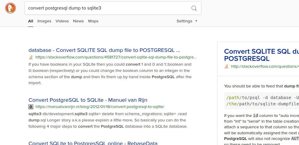
The investigation shows us that there are multiple good approaches to take. We can use a plethora of ways to convert the format - and besides that, the language that we are using is the same SQL in both cases... But there is a problem lurking ahead.
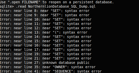

The thing about SQL dialects is that they are very different. The languages look so similar – but what would work, say, MySQL, may not work on PostgreSQL – or the aforementioned SQLite. The language base, of course, is still the same, and a good amount of cases will work just fine. It’s not the same, as, say, expecting Javascript code to run as Java or vice versa.
The thing is, in our case it did not work. Let us proceed to Plan B then.
Plan B: PostgreSQL and Psycopg2
Let us host a server.
There’s a lot of documentation for quick installing, it is pretty easy (surprisingly so, even). Simply running a couple commands we get a server. And the library psycopg2 (a simple one, I promise!) allows us to work with PostgreSQL servers. Maybe with others, the author has not tried – but definitely with PostgreSQL.
Let us write a query then.
Each introduction to SQL you will find online will tell you one thing. It will tell you that the main cornerstone of SQL is the following statement:
SELECT * FROM table
It gives us everything that we have in table.
So let us try running this.
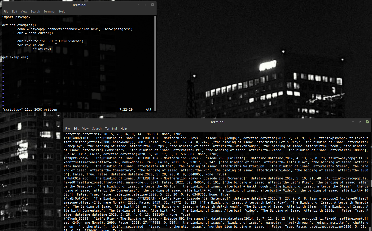
The code is at the top, and the output is at the bottom. It looks nice.
Instead of * in our example we can put a column. Or several columns. That way we can gather only the data that interests us.
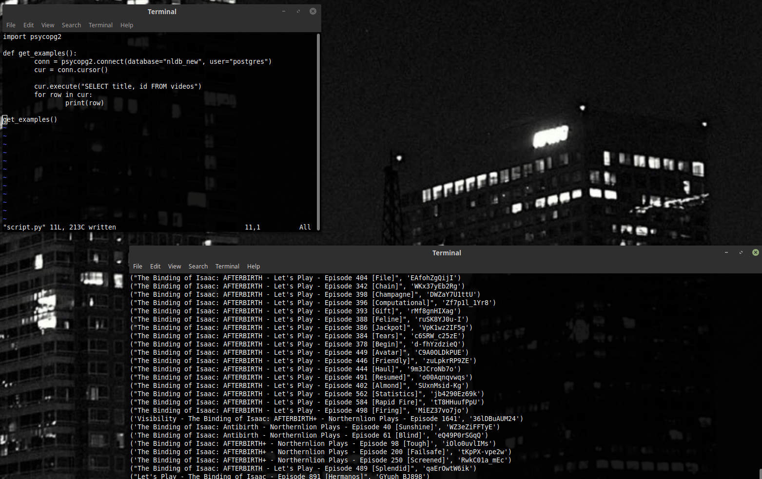
Like that.
If we look at our table a bit more closely, we will see that it contains IDs. Those IDs can help us find an element in a different table.
For example, let us write a script that for each playthrough (one table) gets the name of the video the playthrough was featured in (from a different table).
We will use something called WHERE, which will filter all rows to give us only ones that match some condition.
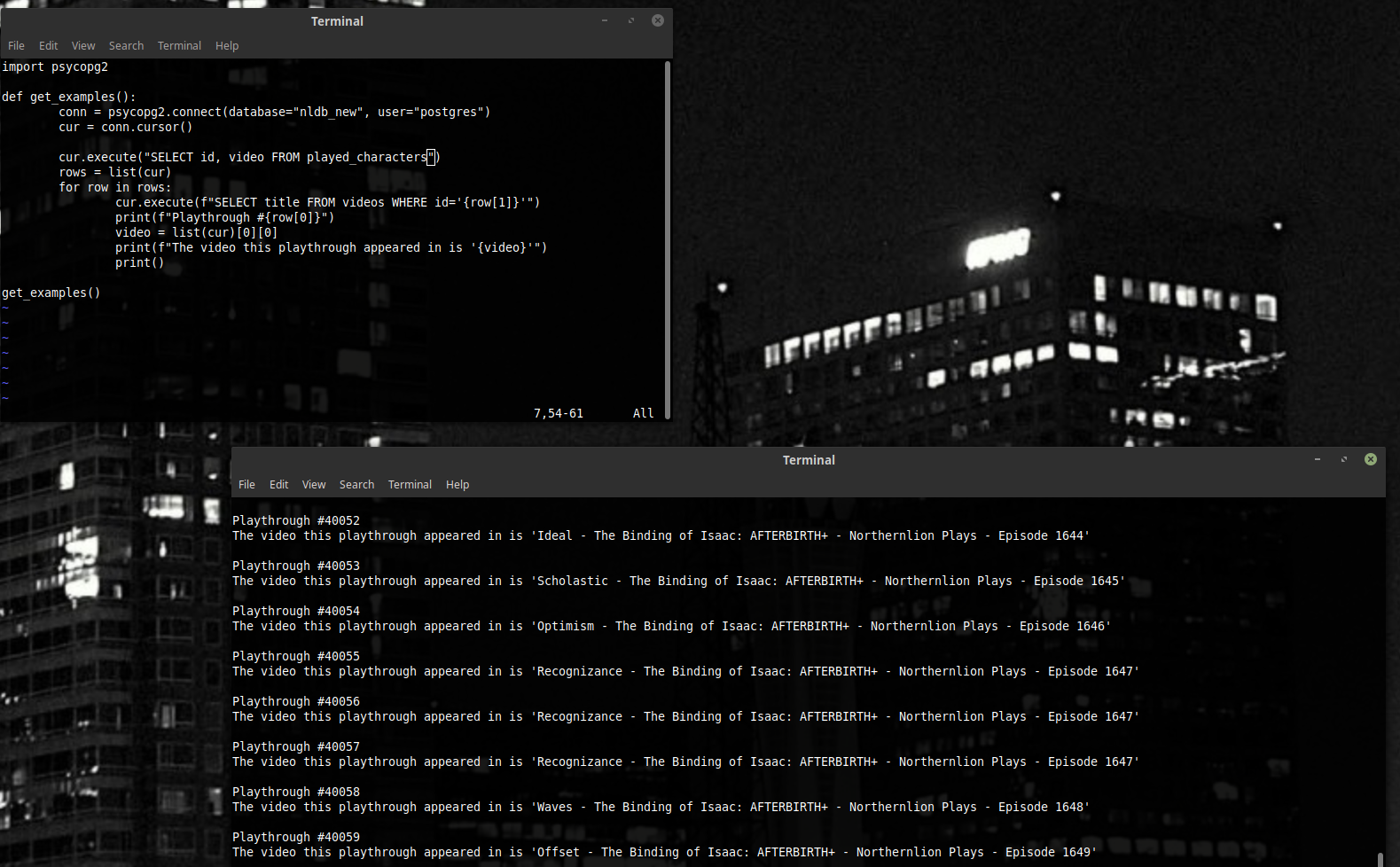
This script here is a horrible, horrible script. Don’t take my word for it, though – just count how many queries does it send to the database (our Postgres that we worked so hard to launch). For each row of our playthrough table, a query to get the video – and one more query to get the playthrough table itself. That’s a lot – poor Postgres! Let us make it into less queries.
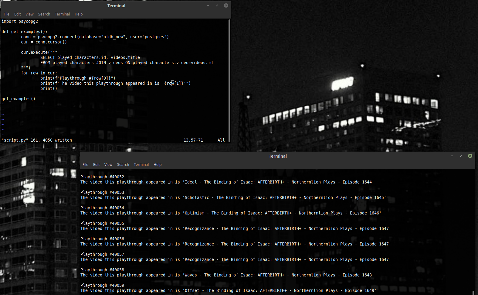
JOIN is a command made just for this situation. It takes a table that has IDs (or any other parameter) pointing to elements of another table, and instead of each ID it puts an entire element there.
There is plenty of nuance there. What if there are several elements with this ID? What if there is none? If anyone is interested in details like this, I recommend taking a look through the documentation. The discussion of such nuance in this article will be limited to looking at a pretty picture and being happy that we made it have only one query. The picture is provided below.
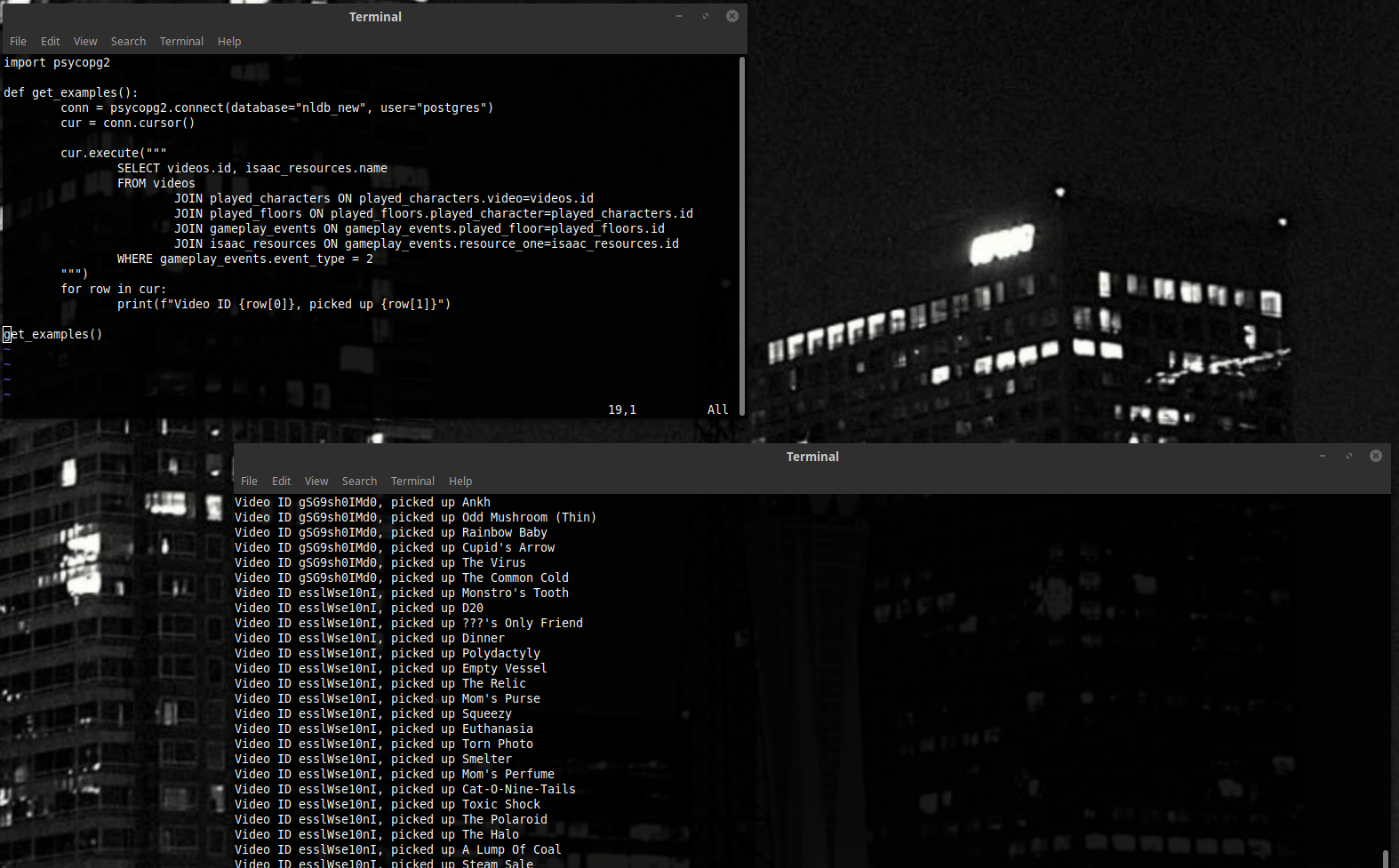
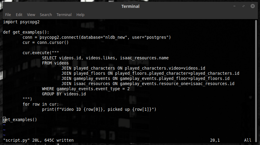
Now, if we want to get a lot of pairs of type (video, name of thing we just picked up),we can use the query below to get it. The meanings of all these fields are talked about in the database documentation – event_type = 2, for example, signifies an event of type “we have picked up an item”. There’s more JOINS in there than we are used to, but the principle works, and we get a really nice result - just what we wanted.
We could stop here. Add another query to get likes for each video, add everything to an array, and live a happy life. But we will not. Let us talk about GROUP BY.
GROUP BY allows us to turn large amounts of rows into one. We have a whole lot of pairs for one video here, for instance. If we turn all those pairs into a single array, our life will be a bit easier. Let’s merge all the pairs with the same videos.id into one row.
(N.B.: This query will not work.)
Why won't it? The answer is simple - we don't know what to do with videos.likes and isaac_resources.name.
When we merge a bunch of different rows, we have to turn a lot of different values into one. Where do we put them then – in an array? But arrays, as per the database’s paradigm, are considered heresy in SQL. Unlike columns, which always have one value (or no value – but that’s a sort of value, too), an array may have multiple values. Maybe five. Or six. Or eight, even. One doesn’t know how much – and that ambiguity is a big problem in MySQL.
For that, GROUP BY is used in tandem with aggregate functions. We can get, for example, the average of all the numbers in a column. The average is one number. Or the sum – one number, too. Not five, not eight. What makes it worse is the fact that different dialects – PostgreSQL, MySQL, SQLite – have different aggregate functions. We are standing right in the murky depths of specification.
Thankfully, despite SQL itself not having the arrays we need, many implementations support at least some version of them. For example, PostgreSQL has the function ARRAY_AGG() - it will unite all the values into an array that we can use.
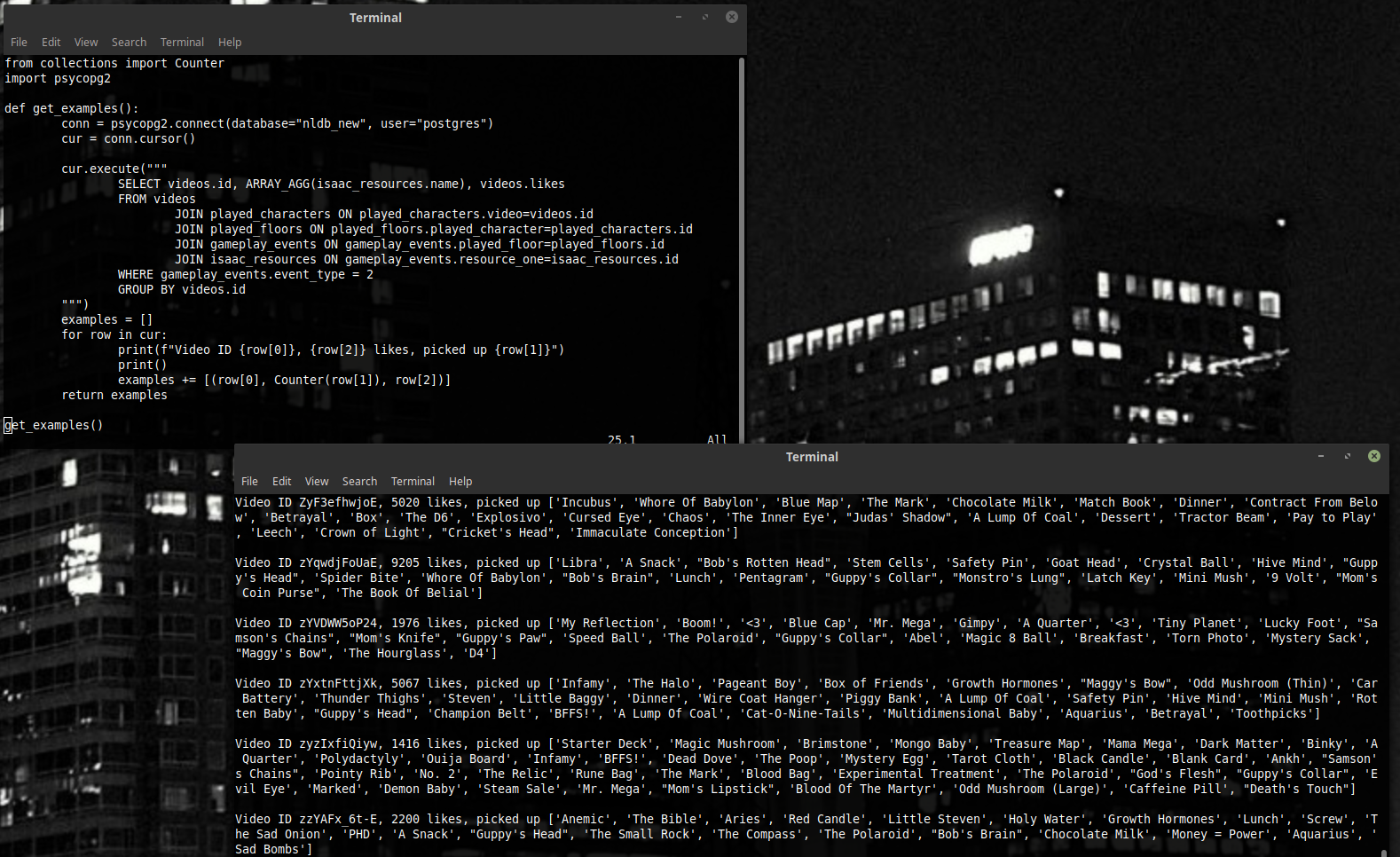
And that’s how we get our examples.
(P.S.: The Counter from the collections module is one great thing, if you want to count something in a simple fashion. Take note!)
3. Machine learning... what is that, anyways?
The way software is usually done is the following: you write code that solves a problem. The harder the problem is, the more complicated code we will have to use. This is software as we know it – familiar to the reader, most likely.
Machine learning gives birth to another paradigm, though – you write code that can learn on examples (or take code that already exists) and then, instead of processing your problem by hand, just feed the machine some examples of the problem you want to solve. Some people call that Software 2.0. Sounds important. More important than it actually is, perhaps? Maybe. Yet people still use it in places. The idea of having a general algorithm you can just punch some data in is very good – at least because finding correlations, especially complicated ones, by hand may be expensive and time-consuming.
We’ll talk about linear regression today. A simple, but rather beautiful method – it will allow us make some predictions for the amount of likes and be happy with how accurate they get.
The idea behind linear regression is the following. You have N situations, and let each have a number correspond to it – the number being the answer we want to know. A number can be of anything – likes, dollars, seconds. We do not discriminate.
Let us say, also, that from each situation we can yank out some values that represent it – its features. A feature can be any number. Or a boolean value – which is, after all, like a number that’s either 1 or 0.
And so, if we give our computer many pairs of type (features, answer), it will look for numbers – weights. A weight for each feature – so that if we sum the products of a feature and its weight for an examples, the number we get would be as close as possible to the right answer. Technically speaking, we minimize the sum of squared differences between answers and scalar products of feature vectors times a common weight vector.
Assuming we already have our weights, let us write a predict function that will give us the answer we expect then.
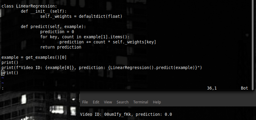
Note also the defaultdict object we are using – taken from the same collections module. It’s really good. It works like a normal dictionary – but if we ask it for a key it doesn’t have, it returns a default value. Like zero in our case. Forget about KeyErrors!
But we have no weights. Where do we get them?
For that, we use gradient descent. It’s pretty simple, too. The big idea is looking which way we should change our weights so that our sum of squares goes down – and just change it in that way repeatedly. If we have some f(x), we subtract from that the gradient of f with respect to x, multiplied by some number – smaller if we want it precise, or larger if we want it fast. A gradient is like a derivative (the slope of a function, the tangent line), but instead of one number, it’s multiple numbers. That’s because we have multiple weights. If we had one weight, it would be the derivative.
Since we don’t want to sum all the examples every step (it’s slow!), a sly trick has been invented. Instead of updating our weight numbers using all the examples at once, we can just take one, or just a bit of examples at once – and update using them. This is stochastic gradient descent, and it is quite good too.
So, what's the gradient of the function we want to minimize for one example? Luckily for us, it just so happens to be the simple difference between our prediction and the answer, multiplied by each of our feature values.
For the first feature, (prediction – answer) * first feature, for the second (prediction – answer) * second feature, et cetera. Counting that is not hard, and descending is not either.
Let us write it.
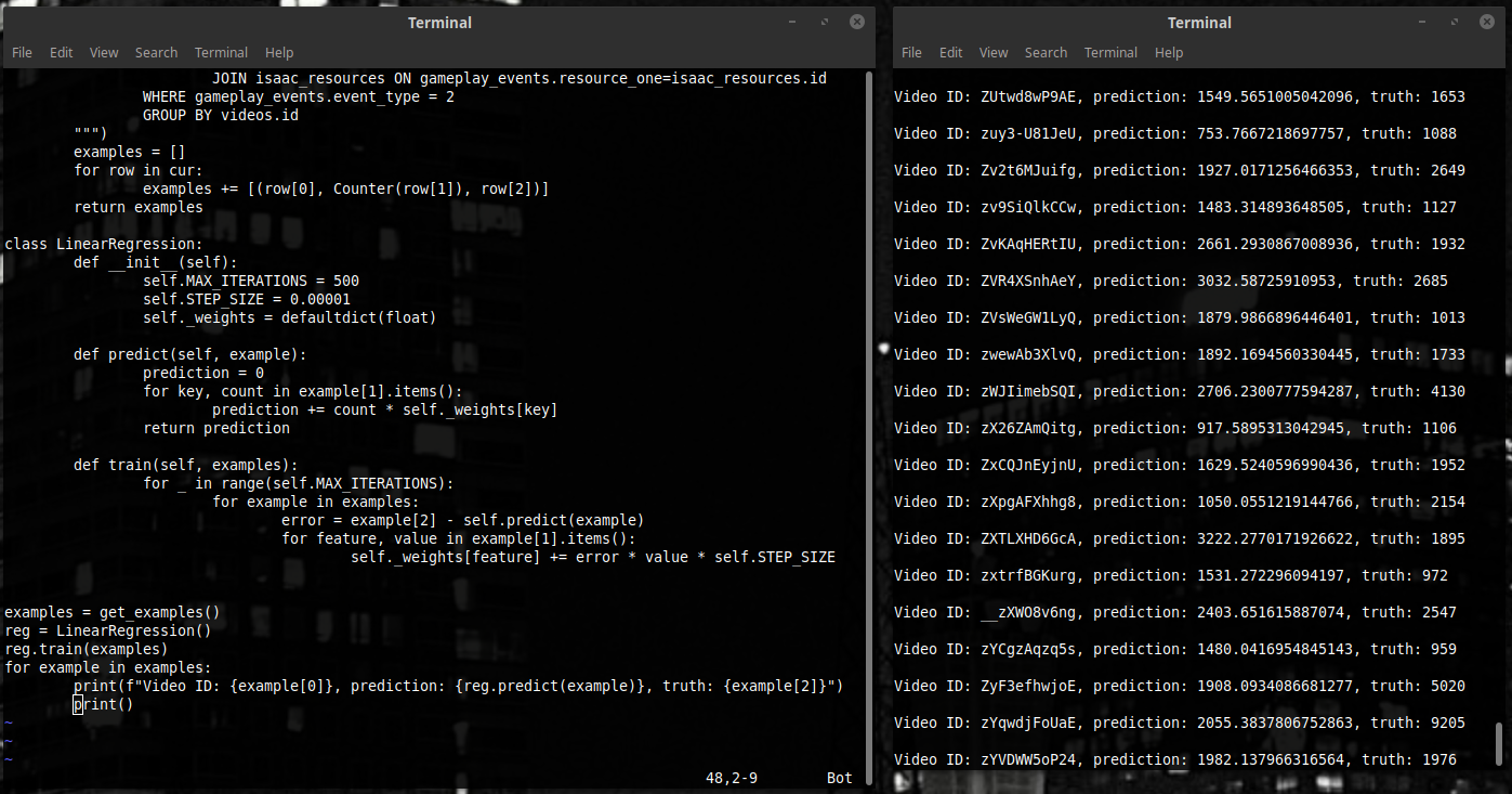
We added the train function - five lines of code. For each example we move weights around so that the square of our difference is a bit smaller. And that’s it – let’s test it.
4. What in the world just happened?
Okay. We have... something. It spews numbers, of some kind. Of course, this is good and all – but that’s not nearly a palatable result. Let’s look at where to dig next now.
First of all, we do not know how to tell if our algorithm is good or not. We have likes and predicted likes. Let us use the difference between the two, the average error.
Second, we give our algorithm all the data when we train it – and when it’s time to test its performance, we give it the same data. When it comes to machine learning, this kind of idea is very dubious. Judge for yourself – if we want our algorithm to work well in general case, what would happen if we gave it the answers? It could learn them by heart – and that would not give us any guarantees on whether or not it would be great at the examples it has not seen. Not a guarantee, but we should avoid that.
For that, what they usually do is they split the examples into three sets: train, validation, and test.
Train is the training set – the one we feed into the train function.
Validation (or dev) is the set that we feed our algorithm to test it. Like a quiz – looking at the results, we see how well is the program handling cases it hasn’t seen exactly. Testing on the training set (train) at the same time is good, too. Usually we look at the average errors on those two sets – we will expect that they both decrease as we train, and train will be a bit less than dev (our program knows it!).
Test is a set we use for final testing. As we write our algorithm, we find many parameters that we can change – the step of our gradient descent, number of different features, and many other things that will not be mentioned in this article. (However, since the name “parameters” in certain terminologies is taken up by things like weights, we call those hyperparameters.)
When we change our hyperparameters, we do so while looking at the dev set and trying to make the error gets as low as possible. But doing it too hard might lead us to becoming dependent on the way our dev set is laid out. If we can lower our error by 0.01% by tuning some knobs, it might not be due to us being awesome hyperparameter experts – might as well just be luck. That’s why when the final result is important, they usually take the third set – and solemnly swear to not test it very often. And if they do, to not tweak hyperparameters based on results.
A toy program such as ours won’t need a test set – but let us introduce the metric of average error as measure of our success, and start tracking it on our two sets.
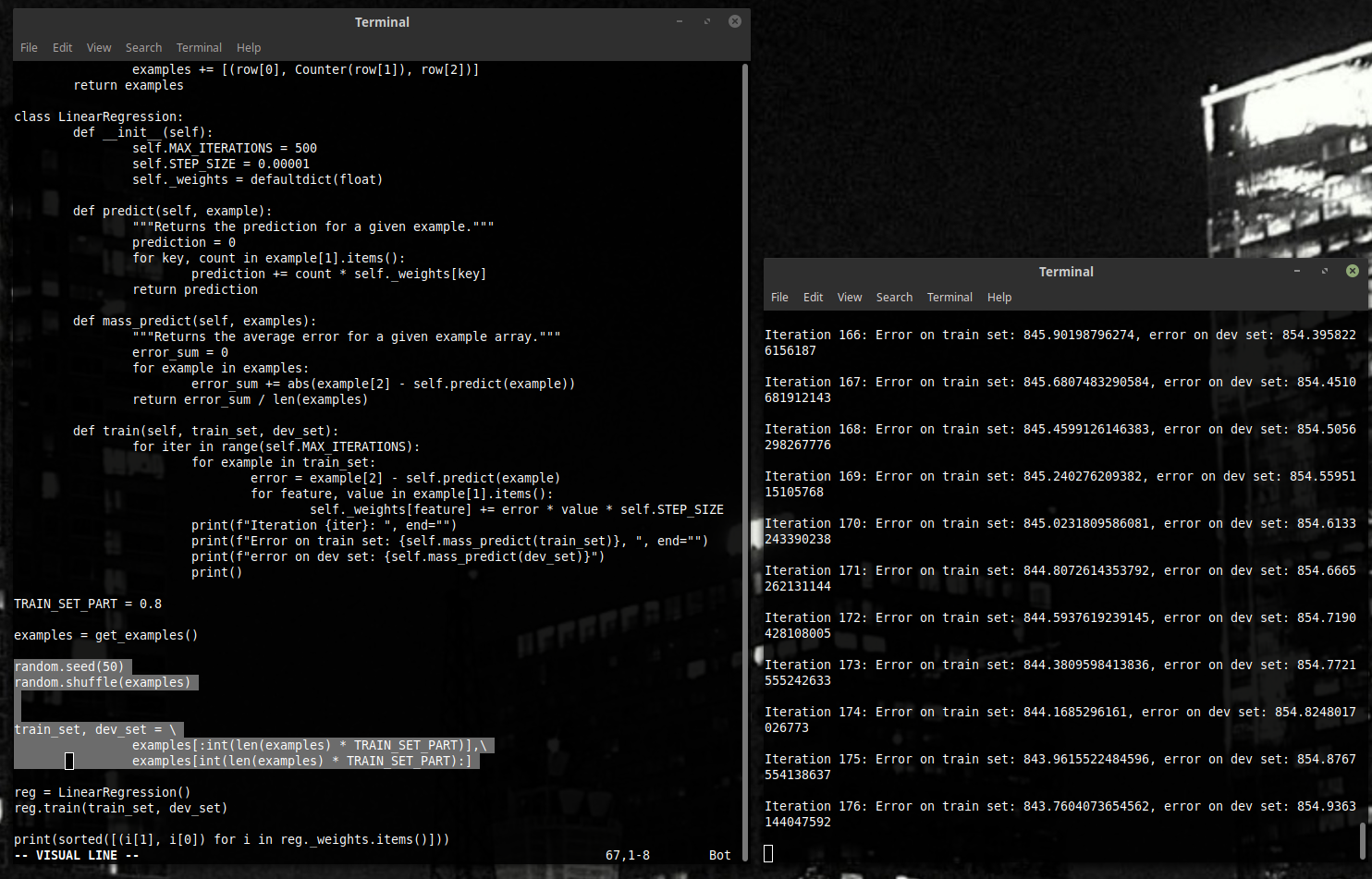
From now on, we will look at the error graph. This one:
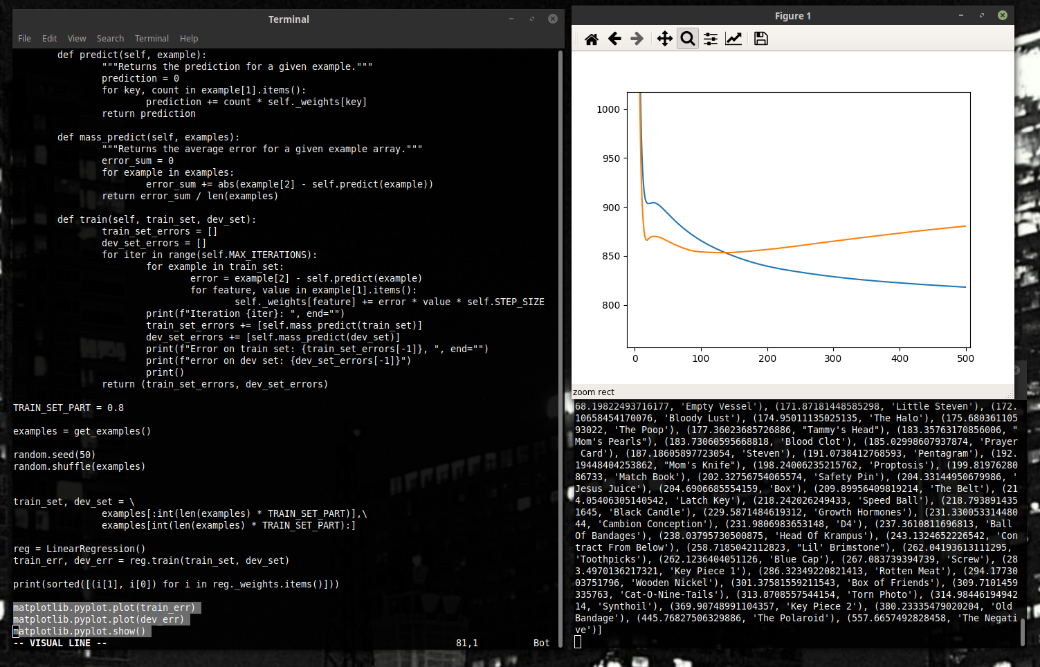
Average dev set error is orange, average training set error is blue..
The console will stop showing anything of interest from now on. Except for the weights. They are quite interesting, actually. However, to understand why, we would need to take quite a bit of a detour into the mechanics of our game and what does picking up certain items mean for the player’s progress. And this is not something that will be done – the article is about machine learning, not The Binding of Isaac gameplay nuance.
To make our graph make a bit more sense, let us look at the average error we would have gotten by just choosing the average number of likes every time. (If we did not know anything about our video, that would be the most efficient way to get a low error.) What is that number? Let’s find out!
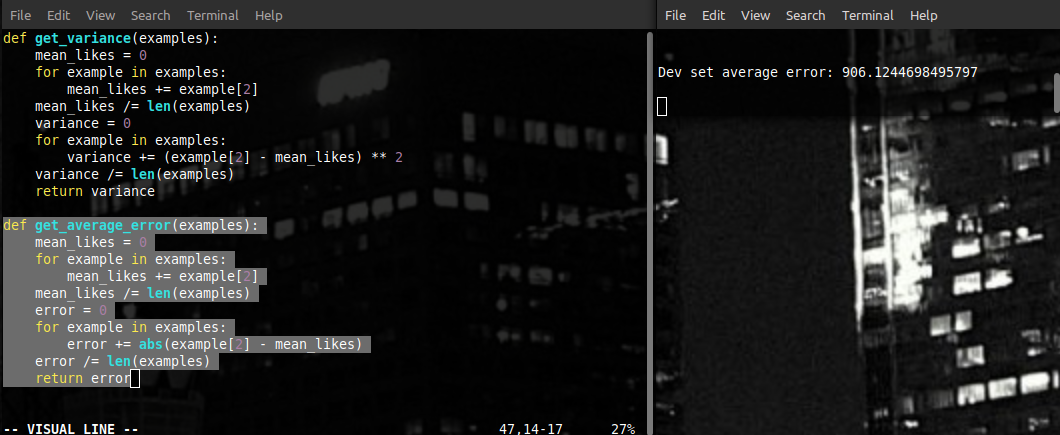
906. And our graph gives us 850 or something in those lines... It’s pretty cool. Remember – we did not show our algorithm a single example from this set. And it just comes out and finds some kind of patterns that make it actually better than random choosing. Now let us optimize this result a bit further.
Remember the beginning of the article? We mentioned the player’s charms as an important factor of the video’s likeability. Why not account for it now? Let’s add another feature, and call it “INTERCEPT” – it will be equal to one in each example. Train the model again, and...
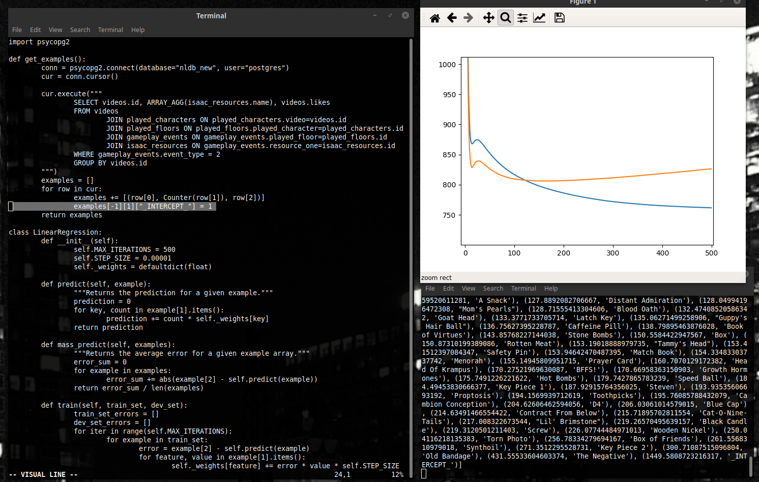
A big downside of our representation at this point is the fact that any video where Northernlion has not collected a single item will always count as having zero likes exactly. To avoid such issues, a popular thing to do in machine learning is to add a dummy feature, equal to one for all the examples. It helps us account for factors that influence all our examples equally.
As we can see, our error is lower now. By 50 likes or so. Progress.
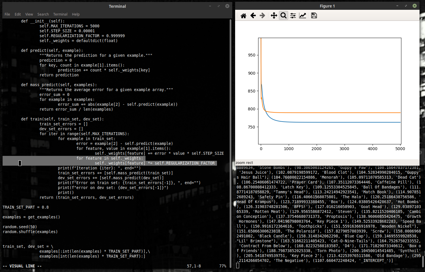
Have you noticed, by the way, how strange our graph looks? As we train, the error on our training set falls – and on our dev set, it rises.
Like in the example below, where we ran it for 5,000 steps instead of 500.

This is a typical case of something called “overfitting”. Leaving the program to look for reason where there is none, we doom it to superstitious beliefs. Trying to explain the fluctuations of the data with its limited set of features, the program invents more and more inappropriate opinions on how the world works. And while on the part of the world we see in the training set, they might work just fine – in the general case, it drifts away from objective reality observed around. Psychologists used to do this sort of thing with pigeons.
The keen eye and the perfect memory of our program are to blame for this orange line going up as it trains. To prevent this from happening, we will need to make our program less sensitive to tiny stimuli. For that, we use something called regularization.
The idea is simple. Our gradient descent, as we described, tries to “pull” the weights towards the spot where the sum of all the squared errors is the smallest. All we have to do is to add another “pull”, this time towards zero.
Mathematically speaking, our loss function (the number that represents how much do we dislike those weights), instead of the sum of squares, becomes the sum of squares plus the norm of our vector (times a constant). The gradient changes accordingly.
One of the simplest ways to do this – after changing the weights, multiply them all by something a bit less than 1. The highlighted lines show this added functionality.
Such a smooth graph might also give us a higher training set error. Finding the right REGULARIZATION_FACTOR is important.
There are, of course, many other methods to improve our result.
We assume a linear dependency here – that is to say, if we find an item twice, it will become exactly twice as fun (or sad) as finding it once. It is, of course, not always the case – that’s why something called binning can be used. Instead of using a number (of objects, say) as the value of our feature, the possible values are divided into several intervals (0, 1, 2-3, 4+) - and then each interval gets its own feature, valued 0 or 1. That way, our feature “item: 3” turns into “item_0:0, item_1:0, item_2-3:1, item_4+:0” – and we can look for patterns based on that.
We could add more features. Our database is big, and many things, fun or not, can happen during a video. But the more features we have, the more combinations of those happen in the wild. The more examples we will need – and the more the chance to overfit.
And the linear regression itself is one of the simplest algorithms around. Ahead lie LDA, Bayesian networks, neural networks of all the different kinds... Machine learning is a deep field, and this article is hardly bigger than dangling your feet over the water from the safety of the shore. Look into the depths, and maybe they will call you. The water is fine.

Will you jump in?
(All code from the article can be found here.)
