VasyaPal Mar 31 2023 at 22:10

GNU radio 802.11 black box optimization

Medium

5 min

2.3K

Wireless technologies*GitHub*Machine learning*

What this all is about

In this post I'll share my experience in adjustment of WiFi physical channel. The channel was implemented on a software defined radio (SDR) platform. WiFi looks like a very complicated thing standardized over hundreds of pages. Could a non-expert with PC and a couple of 100$ devices somehow improve it?

I tried to answer the question experimentally. Gaussian processes were engaged to process noisy and time-consuming channel quality measurements. The work results could be used to finely adjust WiFi channel quality. Project code is available at https://github.com/KVasya/AdjustableWiFi/tree/gpflow .

Software and hardware involved

My experiments were based on GNU radio (GR, https://www.gnuradio.org/) implementation of IEEE 802.11 protocol (aka WiFi, https://github.com/bastibl/gr-ieee802-11 by Bastibl). GR enables you to configure a relatively cheap radio device for WiFi signals. The gr-ieee802-11 implementation in principle reveals all the internal stages of WiFi signal treatment. If we wanted to optimize it, a decent way would be to go deep into the project and see what's going on with the signal. A different way is to consider WiFi implementation as a black box and optimize it's performance by trying many different project parameter values. This way one actually works with a project facing it for the first time. My intention was to find a mathematical framework for such a triage of complicated GR projects. If useful, such a functionality could be wrapped in a standard GR block.

I took 2 HackRF devices (one for transmissions and one for reception, Fig. 0) and changed gr-ieee802-11 into echo configuration: a short text message is encoded into physical signal, sent through transmitting device, then it's caught by receiving device, and then decoded back into text (GNU radio project is shown in Fig. 1). The devices operated in 2.4GHz WiFi frequency range.

Figure 0. Experimental setup. Two HackRF (https://greatscottgadgets.com/hackrf/) devices connected to host notebook PC.

Figure 1. GNU radio project gr-ieee802-11 changed to echo configuration.

The fraction of messages received is a measure of channel quality, it's to be maximized. I took five parameters for optimization, these were: frequency, sensitivity of encoder/decoder, transmitter's IF gain, receiver's IF and VGA gains. The importance of optimal gain is generally obvious. Too low gains mean noisy signal, whereas too big gains lead to nonlinear distortions. In what follows we don't care about what IF or VGA means -- let it be just terms for HackRF physical constituents. Frequency allowed is a separate parameter set by IEEE 802.11, it controls interference with WiFi sources external to the project. From now on these five variables are just floats, bounded withing finite intervals.

Via zmq interface I sent/received messages to/from GR project. Although it's possible to incorporate Python functions or modules into GR project, I preferred to control the project from external script. This way I managed to send not more than one message per 10ms. Another limitation of the project was relatively low fraction of messages successfully passing through the channel, it was ~ 3% at best. As a consequence the measurements of the channel quality were either too noisy or prohibitively time consuming. In some cases (perhaps not exactly this one) optimization can't take too long due to temporal drifts, such as variations in external WiFi sources intensities. To tackle the problem appropriately I resorted to slightly complicated Gaussian processes (GP). Technically I used gpflow Python package for the work, https://github.com/GPflow/GPflow .

Gaussian Processes optimization

GP is a model of an optimized function in parameter space . Scalar channel quality value is measured at parameter vector $\vec{x}\in X$ . In simplest setting, all channel quality measurements at different points in are organized into single vector $\vec{Y}$ distributed as multivariate Gaussian. It's covariance matrix comprises distance dependent term $K(\vec{x_1},\vec{x_2}) = K(||\vec{x_1}-\vec{x_2}|||)$ plus constant diagonal term $\Sigma$ . It practically means that our measurements are noisy at every single point $\vec{x}$ , values of measurements at neighboring $\vec{x}$ -points being statistically dependent. With covariance matrix known, and given some measurements of already taken we could tell the values at unknown points, with some uncertainty. To predict anything useful, a GP model should be initialized first, i.e. we need to feed it some valuable measured points to estimate covariance matrix. Thus initially parameter space is sampled randomly, until we find a few useful points (we get there non-zero channel quality). To be more certain, vanilla squared exponential kernel was used, $K(r) = A*\exp(-\frac{r^2}{\lambda^2})$ , thus we've got three learnable parameters: $\Sigma$ , , $\lambda$ .

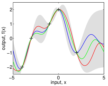
Now suppose we've got GP model initialized. To predict values at new points in , posterior distribution is derived with Bayes formula from Gaussian distribution. Luckily it's also Gaussian with mean and variance, both dependent on previous points sampled. In parameter space the variance (uncertainty) falls close to measured values and rises aside, the mean varies on the distance scale of $\lambda$ . Fig.2 exemplifies posterior distribution in the case of one-dimensional parameter space.

Figure 2. Posterior distribution of GP for 1D parameter space. Crosses mark points with measured values. Shaded areas represent uncertainty of values. Possible (of substantial probability) GP realizations are drawn with colored line within uncertainty area. The image was borrowed from http://gaussianprocess.org/gpml/chapters/RW2.pdf

Given posterior distribution one might choose what $\vec{x}$ should be tried next. There's a bunch of strategies here, and it happened for the problem in case that 'conservative' criterion is suitable, i.e. we took the value with largest $\mu(\vec{x}) - \sigma(\vec{x})$ . In other words, point with largest worst case value is preferred. After getting at new point $\vec{x}$ the GP model is fit again and the process repeats, until we're pretty sure about uncertainties all over the parameter space . For further details on GP see a great resource http://gaussianprocess.org/, particularly a brilliant book http://gaussianprocess.org/gpml/).

Results

Several complications happened in the course of project development, they should be noted.

Frequency was excluded from search space. Although gr-ieee802-11 implementation allows frequency to be changed continuously, channel qualilty degrades very quickly away from a discrete comb of values set by 802.11 standard. The comb structure complicates parameter space and needs a specific approach, e.g. GP kernel might need separate length scale for frequency.
GP process in vanilla form assumes Gaussian with constant zero mean. To improve model quality it's profitable to subtract the mean from values being optimized. Also, scaling of input space to unit intervals over each variable is necessary for GP optimization (otherwise squared exponential kernel has vanishing gradients).
The noises observed aren't exactly Gaussian distributed, especially for quick channel measurements. It's seen even from the fact that they are integer, which seems important at values ~1. The filtering of ~1 and zero values gave poor results. To learn it's parameters correctly GP needs to see zeros and ~ones as well.

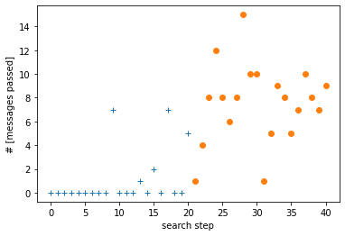
Here is an example of optimization sequence, Fig.3. First -points were taken randomly until 5 points with non-zero channel qualities appeared. Last ... points were taken via model conservative predictions and show considerable improvements over the random search.

Figure 3. Plot of channel quality (quantity of messages echoed out of 1e03 sent) vs. search step. Crosses label the points of random search stage, it continued until 5 points with non-zero values were accumulated.Circles denote points derived from GP model search.

It's interesting to analyze the convergence of 20 last points prescribed by GP model, in Fig. 4. It looks like the points oscillate due to noises in channel quality measurements.

Figure 4. Normalized distance of points in GP guided search to the final point of the search. Normalization maps coordinates to [-1,1] intervals.

Conclusions

An approach for internals-agnostic GNU-radio project optimization was tried and gave some positive results. It's applicability to arbitrary project is out of question at the time, as difficulty with frequency optimization demonstrates. GP apparatus seems to be a promising tool for noisy 'little' data, but it requires careful adjustments of kernel and sequential search strategy.

Tags:

Hubs: